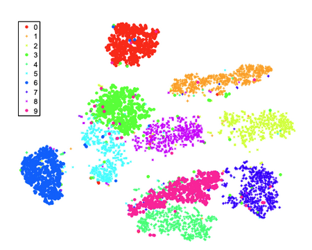
t-distributed Stochastic Neighbor Embedding says "what"
Contents
What is t-SNE

t-SNE or t-distributed Stochastic Neighbor Embedding (Maaten and Hinton 2008) is a dimensionality reduction technique that projects data onto lower dimension (typically 2 or 3) based on a normal distribution for the initial similarity derivation and then a t-distribution for the projected space. The perplexity controls the scaling of the normal distribution used for comparing similarities.
The algorithm preserves clustering, but distorts original distances (as any dimensionality reduction technique would).
Perplexity
Perplexity can be intuitively thought of as the following: expected density around each point; (loosely as) how to balance attention between local and global aspects of your data; a guess about the number of close neighbors each point has.
Perplexity is a key parameter of t-SNE.
- Balances local & global aspects of data
- Low values empharize local structure, while high values emphasize global structure
- A guess about number of close neighbours each data point has
- Number of points to compare to each other
- Recommended range - 5-50
Please use this beautiful interactive blog post “How to Use t-SNE Effectively” (Wattenberg, Viégas, and Johnson 2016) to play around with the parameters of t-SNE. Our good friend at StatQuest (StatQuest with Josh Starmer 2017) also has a 12 minute explanation of t-SNE.
Normal to t
The reason for first using a normal distribution and then a t-distribution is to avoid clumping the points in the projected space as the t-distribution is a bit more thicker at the tails thus providing a bit more slack for the lower similarity points.
The Algorithm
It proceeds as follows:
- Determine unscaled similarity between all points and point of interest based on original t-distributions based on a perplexity value
- Do this for any point from selected point
- Iterate over all points
- For each point scale similarities so they all add up to one (dividing by sum of unscaled similarity scores)
- Average simality score for each point (in and out)
- Get matrix of similarity scores.
- Project randomly onto desired number of latent dimensions
- Repeat 1-8 on projection 7 but this time with a t-distribution to derive similarity matrix
- Make matrix derived in 8 converge to the matrix derived in 6 in tiny steps with epsilon learning rate by moving points with higher similarity closer and lower similarity further to each other.
Example in Python
A simple t-SNE example (supply a df with text column) with TF-IDF sentence vectors. Can be repeated with fastText embeddings or on Orange Data Mining for quick PoCs. The example below creates a nice plotly chart with text that is wrapped at 20 chars.
from sklearn.feature_extraction.text import TfidfVectorizer
from sklearn.manifold import TSNE
import plotly.express as px
import textwrap

# Create a TfidfVectorizer object
vectorizer = TfidfVectorizer()

# Fit and transform the text column
tfidf_matrix = vectorizer.fit_transform(df['text'])

# Create a DataFrame with the TF-IDF scores
tfidf_df = pd.DataFrame(tfidf_matrix.toarray().mean(axis=0))
# tfidf_df
tfidf_df = tfidf_df.set_index(vectorizer.get_feature_names_out())

tfidf_df.reset_index(inplace=True)
tfidf_df = tfidf_df.rename({"index":"token", 0:"tfidf"}, axis=1)

tsne = TSNE(n_components=2, random_state=0)
tsne_results = tsne.fit_transform(tfidf_matrix.toarray())

def wrap_text(text, width=20):
    return "<br>".join(textwrap.wrap(text, width=width))

# Apply text wrapping to the text_column
df['wrapped_text'] = df['text'].apply(wrap_text)

df['tsne-2d-one'] = tsne_results[:,0]
df['tsne-2d-two'] = tsne_results[:,1]

# Create an interactive plot
fig = px.scatter(df, x='tsne-2d-one', y='tsne-2d-two', hover_data=['wrapped_text', 'score'], color='label')

fig.update_layout(
    xaxis=dict(
        scaleanchor='y',
        scaleratio=1,
    ),
    yaxis=dict(
        scaleanchor='x',
        scaleratio=1,
    ),
    width=800,  # Width in pixels
    height=800  # Height in pixels, set the same as width for a square aspect ratio
)

fig.show()

fig.write_image("t-sne.png")
t-SNE traps
Avoid the trap where low perplexity leads to a perception of patterns where none exist. Strike a fine-balance between local and global structures. Observing consistent patterns across multiple runs with different random initializations will strengthen the interpretation.
References
Maaten, Laurens van der, and Geoffrey Hinton. 2008. “Visualizing Data Using t-SNE.” Journal of Machine Learning Research 9 (86): 2579–2605. http://jmlr.org/papers/v9/vandermaaten08a.html.
StatQuest with Josh Starmer, dir. 2017. StatQuest: T-SNE, Clearly Explained. https://www.youtube.com/watch?v=NEaUSP4YerM.
Wattenberg, Martin, Fernanda Viégas, and Ian Johnson. 2016. “How to Use t-SNE Effectively.” Distill 1 (10): e2. https://doi.org/10.23915/distill.00002.